Part 2 – in which I acknowledge an embarrassing misunderstanding of the data.  Yeah, about that…  My previous post about how the proper way to assess Medicaid’s effect on patient-level quantities like GH level would be to examine a correlation plot of GH levels and the start and end of the experiment?  Can’t be done.  Can’t be done because there is no baseline data.  It’s right there in the Methods summary:

Approximately 2 years after the lottery, we obtained data from 6387 adults who were randomly selected to be able to apply for Medicaid coverage and 5842 adults who were not selected. Measures included blood-pressure, cholesterol, and glycated hemoglobin levels…

I just presumed there was baseline data.  Nope.  Reading comprehension shortcoming on my part.  (Thanks to Austin Frakt and the lead study author Katherine Baicker for politely pointing that out to me.  Yah.  Nothing like demonstrating one’s ignorance in front of people who know what they’re doing.  Moving on…)  Lack of baseline data certainly complicates interpretation of the t=2 years data.  I maintain that comparison of before and after measurements is what you’d like to use as the basis for your conclusions but, to appropriate a line from Rumsfeld, “You analyze the data you’ve got not the data you’d like to have.”

[ADDENDUM:  I’m also reminded of John Tukey’s line:  “The combination of some data and an aching desire for an answer does not ensure that a reasonable answer can be extracted from a given body of data.”]

So, where am I at now?  I’m still adhering to the maxim, “When you don’t know anything do what you know.”   Taken at face value, one might interpret that as an invitation to do nothing.  It is not.  It’s a suggestion that when don’t know the proper way to tackle a problem then you should apply the tools you know.  Write an equation.  Make a prediction.  Examine how your prediction deviates from the observation.  The thought is that by determining the cause for the deviation between prediction and observation you’ll learn how to address the problem correctly.

With that in mind, I started off looking at this as a rate estimation and comparison problem.  Why?  Because I had information in front of me which made it easy to estimate high GH rates and compare them.

• Sample 1 (treatment group):  n1=6387, rate of high GH = r1 = 5.1% so k1 = 0.051*6387 = 326
• Sample 2 (Medicaid recipients):  n2=1691, rate of high GH = r2 = 4.17% so k2 = 0.0417*1691 = 70

(The sample size is ni and the number of occurrences of the effect is ki.)  My approach was to calculate probability distribution functions (pdfs) for r1 and r2 and then calculate the probability that r1 > r2 from the estimated pdf.  (The concept is legit but there are problems in the details of how to apply the concept here.  That’s important to keep in mind but I’ll continue down the path for the sake of illustrating my thought process.)  The variance in the calculated rates is trivial to compute from the information provided:

The sample sizes are large so I can approximate the pdfs as Gaussians with standard deviations equal to the square root of the variance calculated above.  Here’s what those pdfs look like:

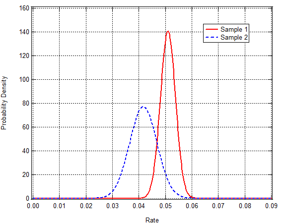
The solid red curve is the estimated pdf for the rate of occurrence in Sample 1 (r1) and the blue dashed curve is the estimated pdf for the rate of occurrence in Sample 2 (r2).  Visual inspection of the curves indicates that there’s a high probability that r1 > r2.  (Unfortunately, with respect the Oregon experiment data comparing r1 with r2 is comparing apples to oranges.  For the moment, never mind what the rates actually correspond to.  Just follow the process.)  What I’m interested in the probability of r1 > r2.   I compute that as the integral of the product of the pdf for r2, , and the probability of exceedance for r1.  (The probability of exceedance, , is just unity minus the cumulative distribution function.)  Here’s a plot of , and their product:

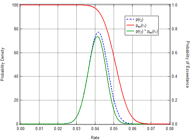
I evaluate the integral and I get 89% probability that r1 > r2.  That’s interesting.  More interesting is the probability that r1 is x times larger than r2.  Here’s the result of those calculations:

My choice of axes is perhaps a bit odd – on the x-axis is the ratio of r1 to r2 and the y-axis is the probability the actual ratio of r1 to r2 is greater than the value on the x-axis.  As noted above, the calculation tells me 89% probably that r2 < r1, 54% probability that r2 is at least 20% less than r1, and 11% probability that r2 is at least 1/3 less than r1.  If I could establish how to correct the estimated rates for instrumental variable effects then I think the approach above would be a constructive way of interpreting the Year 2 GH observations.  That said, I don’t know how to do that correction.

My homework:  A correspondent was kind enough to forward the Appendix to the Oregon paper as well as the authors’ paper (plus appendix) describing their Year 1 findings.  I’ve only skimmed it, but the Appendix to the recent paper describes the authors’ methodology.  I should digest that before proceeding.