Quantitative election forecasters received a lot of attention in the popular press this year. Nate Silver and his “538” blog at the NY Times probably received the most but Sam Wang, Drew Linzer and others also got their fair share. Prior to the election, I only followed Silver and, to a lesser extent, Wang. Both predicted an Obama victory but Wang gave him a much higher probably of victory than did Silver.
Now that the results are in, there’s a fair amount of interest in determining who was most accurate. (See, e.g., here and here.) Silver and Linzer presented their predictions in a manner which makes them easier to evaluate than the others – easier for me at least. (Credit to them for doing so.) A.C. Thomas does a nice compare and contrast here and concludes that Silver’s predictions are higher fidelity, i.e., they’re accurate and, at least as significant, he appears to have the uncertainties associated with his predictions nailed. Thomas was gracious enough to make the data he used in his analysis publicly available here. I worked the numbers and – not surprisingly – saw the same things he did. I also noted a few other things.
First off, the data and how I worked it: As noted above, I used the data A.C.Thomas made available – Silver and Linzer’s predicted Obama and Romney vote percentages for all fifty states. (Third party votes are not included in the analysis.) They both made specific predictions and provided associated uncertainties. Both their models were quite accurate – both were good to about +/-2%. What I’m more interested in is how well they estimated the uncertainties associated with their predictions. Did they get the scale right? In order to do so, I calculated z-scores from the actual vote totals, their predictions and the associated uncertainties:
z = (actual Dem share – predicted Dem share)/sigma.
I then calculated the median z and normalized median absolute deviation (nmad) of z. Median z is a measure of bias and nmad is an indicator of how well they estimated their uncertainties (I use median and nmad rather than mean and st.dev. because the former are less sensitive to outliers than the latter. The definition of nmad is: nmad = median{abs(z – median(z))}/0.6745.)
If their predictions were unbiased then median(z) would be approx. zero. If prediction error were normally-distributed and they got the st.dev. right then nmad would be approx. unity. The results:
Silver: median(z) = 0.42, nmad = 1.01
Linzer: median(z) = 0.26, nmad = 1.42
Median(z) > 0 means predictions are GOP biased. Silver’s median(z) indicates that the bias was 0.42 of his self-declared standard deviations – pretty modest. For comparison, Linzer’s predictions were GOP-biased by 0.26 of his self-declared standard deviations – even more modest than Silver’s.
What the nmad values tell me:
1) Silver appears to have his uncertainties nailed
2) The uncertainties associated with Linzer’s predictions appear too small by a factor of about 1.4.
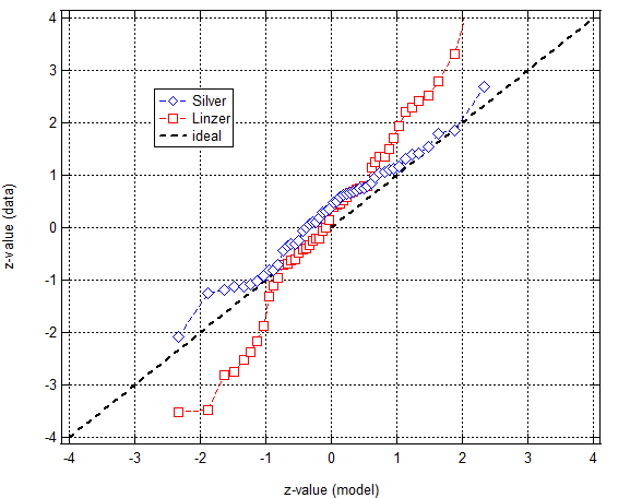
You can see this in a Q-Q plot:
The points from Silver’s predictions lie pretty close to the one-to-one correlation line whereas the line (roughly) defined by Linzer’s points are too steep – too steep by a factor of about 1.4. (The slope is what matters when assessing the scale of uncertainty estimates. Offsets are due to bias.)
Interestingly, if you inflate Linzer’s sigma values then recompute p-values Linzer’s predictions look much better. I don’t know what to make of the factor of 1.4 though. I just read his 2012 paper on the 2008 election but haven’t looked closely enough at his analyses to say whether the factor of 1.4 could be explained away by an atypical definition of confidence limits or the like.

